HSP Desktop — User Manual
Version: 1.0.0 · Technology: HSPiPy v1.1.8
Table of Contents
1. Introduction
HSP Desktop is a desktop application for computing and visualising Hansen Solubility Parameters (HSP). It lets you build a solvent dataset, score each solvent for compatibility with a material of interest, fit an HSP sphere (or two spheres simultaneously), and instantly see the result in an interactive 3D or 2D plot.
The science is powered by HSPiPy, a Python library that implements the HSP sphere optimisation algorithm. The application wraps that library in a native desktop interface available for Windows, macOS, and Linux. By purchasing HSP Desktop you directly support the continued development of HSPiPy as an open-source project.
Key capabilities:
- Access to a built-in database of hundreds of solvents with full HSP data
- Manual scoring of solvents on a 0–6 scale
- One-click HSP sphere fitting with accuracy and DATAFIT metrics
- Simultaneous fitting of two HSP spheres
- Surface Explorer: find database solvents near the sphere boundary and add them to the grid
- Solvent gradient generation (blends of two solvents at variable ratios)
- Import from
.csv,.hsd, and.hsdxfiles - Export to CSV or Excel
- Save and reload named grids from a local database (fit results are saved alongside the grid data)
- Interface available in English, Chinese (简体中文), and Spanish (Español)
2. Installation & First Launch
Installation
Double-click the installer (.msi on Windows, .dmg on macOS, .deb on Linux) and follow the on-screen steps. The application installs to your user directory and does not require administrator privileges.
Security warnings (unsigned app)
HSP Desktop is currently distributed without a platform code-signing certificate. Your operating system will show a one-time security warning the first time you install or open the app. This is expected — follow the steps below to proceed.
When you see "Windows protected your PC":
1. Click More info
2. Click Run anyway
macOS will block the app on first launch. Depending on your macOS version you may see either "cannot be opened because the developer cannot be verified" or "is damaged and can't be opened". The fastest fix for both is to run this command once in Terminal after installing, then relaunch the app:
xattr -cr /Applications/hsp-desktop.appIf you see the "cannot be verified" dialog (not the "damaged" one), you can alternatively go to System Settings → Privacy & Security, click Open Anyway, and relaunch. The xattr command works for both cases and is always safe to run.No extra steps are required for the
.deb package.If you run into any trouble during installation, contact support@g-npd.com.
Splash Screen
When the application opens, a splash screen is displayed. On first launch, a setup dialog guides you through three steps: language selection, reviewing the License Agreement (EULA), and license activation. A progress indicator at the top of the dialog shows which step you are on, and you can go back to the language step at any time by clicking Back on the EULA step. Once all steps are completed, the backend starts automatically and an animated progress bar with rotating status messages confirms that startup is in progress. On most systems this takes 3–10 seconds; on macOS the very first launch may take a few extra seconds while the system verifies the backend component. A Cancel button is shown at the bottom — clicking it quits the application cleanly.
If the Backend Does Not Start
The app polls the backend continuously with no fixed timeout, so a slow machine will still succeed given enough time. If something is genuinely wrong, click Cancel to quit and try the following:
- macOS only — run
xattr -cr /Applications/hsp-desktop.appin Terminal, then relaunch. - Check that port 8000 is not already in use by another application.
- Relaunch the app — if the backend crashed on the previous run it may have left a stale process.
- Contact support@g-npd.com and include the backend log (click Retry then Refresh Log in the error panel).
2.1 Language Selection
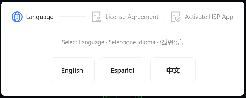
On first launch, a setup dialog appears with a three-step progress indicator at the top. The first step asks you to select your preferred interface language.
Click one of the three options — the dialog immediately advances to the next step. If you need to change your selection, click Back on the EULA step to return here.
The selected language is remembered for all future launches and can also be changed at any time in Settings.
2.2 License Agreement (EULA)
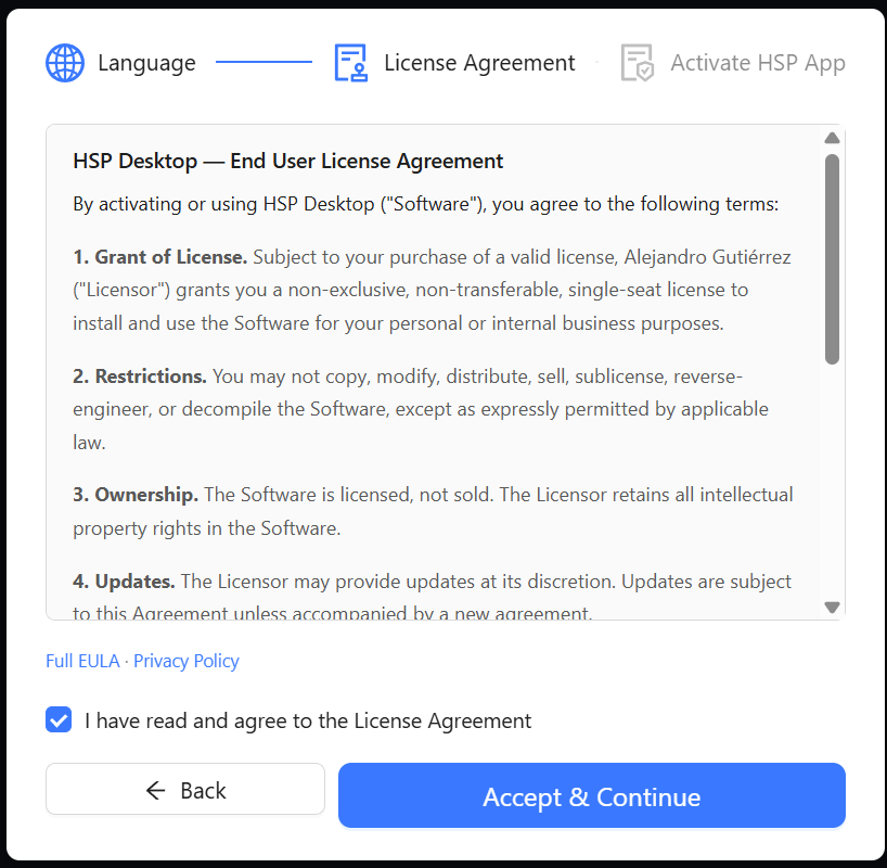
The second step shows the End User License Agreement. You must:
- Read the End User License Agreement (scroll through the text box).
- Tick the "I have read and agree to the License Agreement" checkbox.
- Click Accept & Continue.
If you selected the wrong language in the previous step, click Back to return to the language selector.
The acceptance is stored locally; this step does not appear again on subsequent launches.
Links to the full EULA and Privacy Policy are provided at the bottom for reference.
2.3 License Activation
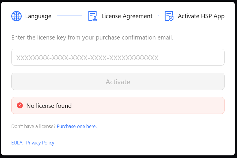
The third step activates your license. If a valid license is already stored on your machine this step is skipped automatically and the backend starts loading.
To activate:
- Locate the license key in your purchase confirmation email (format:
XXXXXXXX-XXXX-XXXX-XXXX-XXXXXXXXXXXX). - Paste or type the key into the input field.
- Click Activate (or press
Enter).
The application contacts the license server to validate the key. Once validated, the dialog closes and the backend starts loading automatically — the progress bar begins and the main interface loads once the backend is ready.
If the key is rejected, an error message is displayed below the input. Check that the key is complete and unmodified, then try again.
3. Interface Overview
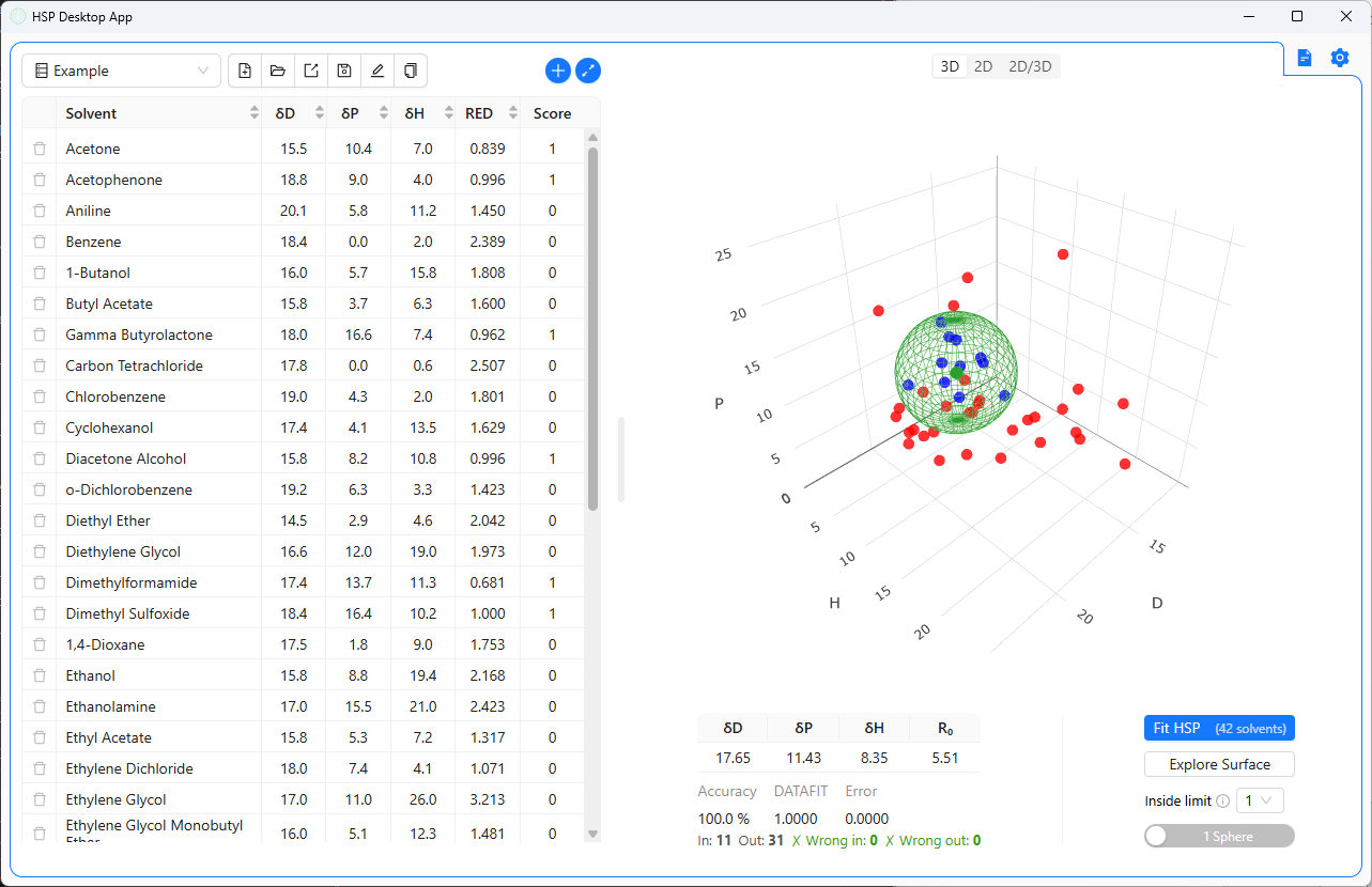
The main window is divided into two resizable panels separated by a drag handle.
┌─────────────────────────────┬──────────────────────────────────────┐
│                             │                          📄  ⚙       │
│   Solvent Grid              │  [ 3D | 2D | 2D/3D ]                 │
│   ─────────────────────     │                                      │
│   Grid selector toolbar     │   3D / 2D Plot                       │
│                             │                                      │
│   ┌─────────────────────┐   │                                      │
│   │ Solvent table       │   ├──────────────────────────────────────┤
│   │ (scrollable)        │   │   Fitting Panel                      │
│   └─────────────────────┘   │   δD δP δH R₀ | Fit HSP | Explore   │
└─────────────────────────────┴──────────────────────────────────────┘
| Area | Description |
|---|---|
| Left — Solvent Grid | Toolbar for grid management + scrollable solvent table |
| Right top — Plot | Interactive 3D or 2D scatter plot of the solvent space |
| Right bottom — Fitting Panel | HSP fitting controls, results, and Surface Explorer |
| Top right — Docs icon () | Opens the user documentation in your browser |
| Top right — Settings icon () | Opens the Settings modal (language, host, port, API key) |
| Top right — Plot mode selector | Switches between 3D, 2D, and 2D/3D views |
You can drag the vertical divider left or right to resize the two panels.
4. The Solvent Grid
4.1 Creating and Managing Grids
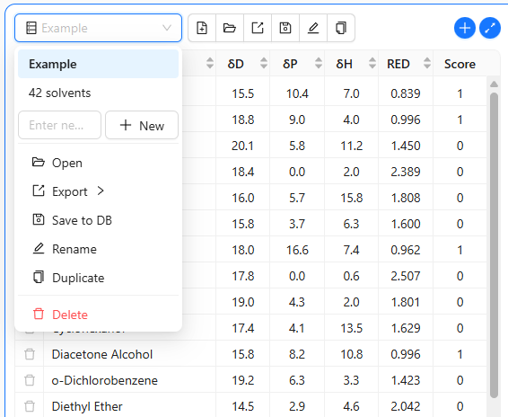
The toolbar at the top of the left panel contains a dropdown selector and a row of icon buttons.
Dropdown selector
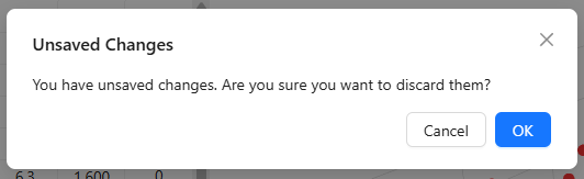
Click the dropdown to see all grids saved in the local database. Click a grid name to load it. If you have unsaved changes in the current grid, a confirmation dialog will ask whether to discard them.
Inside the dropdown there is also an inline area to create a new grid: type a name in the text field and press New.
Icon buttons (left to right)
The icon buttons are quick-access shortcuts to the most common actions also available inside the dropdown menu.
| Icon | Action |
|---|---|
| Create a new empty grid | |
Open a file (.csv, .hsd, .hsdx) | |
| Export the current grid (hover to choose CSV or Excel) | |
| Save the current grid (and current fit results) to the local database | |
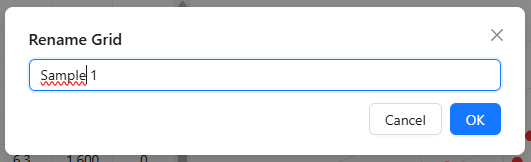
| Rename the current grid | |
| Duplicate the current grid |
The save icon turns amber when the grid has unsaved changes.
When a grid is saved, the current HSP fit results (if any) are stored alongside the solvent data. They are automatically restored when the grid is reloaded.
Grid actions inside the dropdown menu
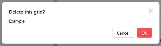
The dropdown also exposes the same actions as labelled text buttons (Open, Export, Save to DB, Rename, Duplicate, Delete), making it self-explanatory if you are unsure what an icon does.
4.2 Adding Solvents from the Database
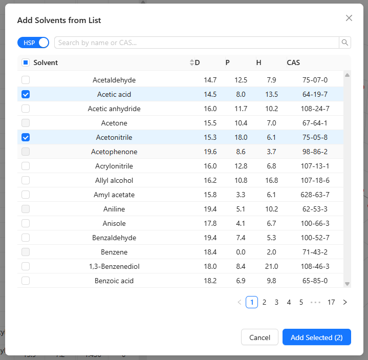
Click the button on the right side of the toolbar to open the solvent picker.
The picker shows the full built-in solvent database. Two features help you find solvents quickly:
- Search bar — type any part of the solvent name or its CAS number; the table filters in real time.
- HSP / FULL toggle — in HSP mode only the columns δD, δP, δH, and CAS are shown; switch to FULL to see additional properties: molar volume, boiling point, molecular weight, viscosity, heat of vaporisation, and SMILES.
Select one or more rows using the checkboxes. Solvents already present in the current grid are shown greyed out and cannot be selected again. When ready, click Add Selected (n) to add them to the grid.
4.3 Adding Solvent Gradients
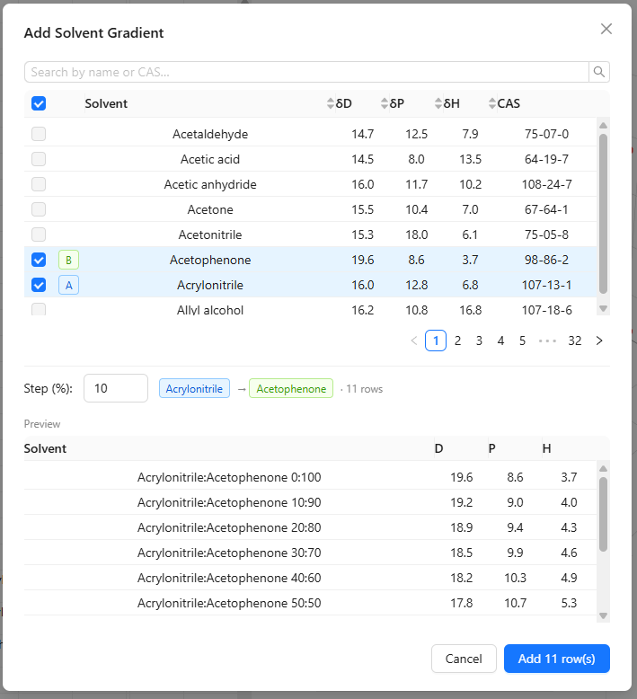
Click the button to open the gradient picker. This tool generates a series of blend rows between two solvents at evenly spaced mixing ratios.
Steps:
- Use the search bar to filter the solvent list.
- Click one solvent to mark it as A (blue tag).
- Click a second solvent to mark it as B (green tag).
- Set the Step (%) value — e.g.
10generates blends at 0:100, 10:90, 20:80, … 100:0. - A preview table shows the calculated HSP values for each blend.
- Click Add n row(s) to insert the gradient into the grid.
The generated row names follow the pattern SolventA:SolventB ratio_A:ratio_B, e.g. Ethanol:Water 30:70.
4.4 Importing Files
Click the Open button (folder icon) to import data. Supported formats:
| Extension | Description |
|---|---|
.csv | Comma-separated values with columns Solvent, D, P, H, Score |
.hsd | HSPiP native dataset format |
.hsdx | HSPiP extended dataset format |
The file name (without extension) is used as the grid name. The imported data is treated as unsaved until you explicitly save it to the database.
4.5 Exporting Data
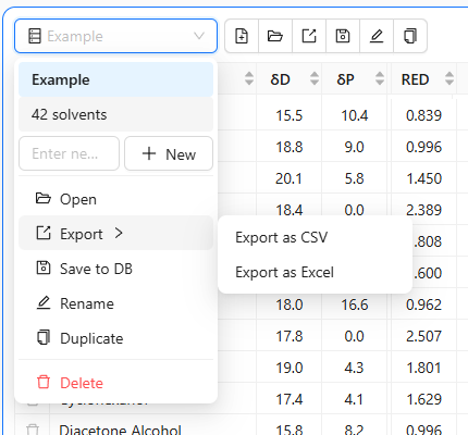
Hover or click the export icon () to choose the format:
- Export as CSV — a plain
.csvfile with all columns including computed RED values. - Export as Excel — an
.xlsxfile suitable for further analysis in spreadsheet tools.
The file is saved to your Downloads folder with the grid name as the filename.
4.6 Scoring Solvents
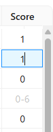
The Score column is the only editable column in the table. It accepts integer values and represents the experimentally observed compatibility of each solvent with the target material.
Two scoring conventions are supported — choose the one that matches your experimental data and set the Inside Limit accordingly (see Section 5.2):
Binary scoring (0 / 1)
The simplest convention: a solvent either dissolves the material or it does not.
| Score | Meaning |
|---|---|
| 1 | Good solvent — dissolves / interacts with the material |
| 0 | Bad solvent — no interaction |
Set Inside Limit = 1 when using this convention.
Graduated scoring (1 – 6)
A finer scale that captures degrees of solubility, following the HSPiP convention:
| Score | Meaning |
|---|---|
| 1 | Completely dissolves |
| 2 | Mostly dissolves |
| 3 | Partially dissolves / swells |
| 4 | Slight interaction |
| 5 | Little to no interaction |
| 6 | Untouched — no effect at all |
Set Inside Limit to the threshold that separates "good" from "bad" for your material.
Keyboard shortcuts in the Score column
| Key | Action |
|---|---|
Enter or ↓ | Move to the next row |
Shift+Enter or ↑ | Move to the previous row |
4.7 Row Colour Coding
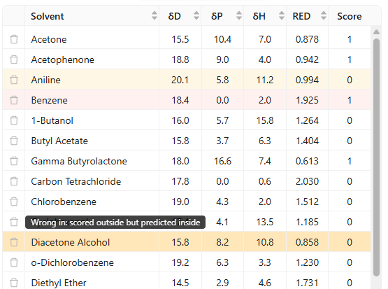
After a fit has been run, rows whose experimental score disagrees with the sphere prediction are highlighted:
| Highlight | Meaning |
|---|---|
| Red background | Wrong in — solvent scored as bad but falls inside the sphere (RED ≤ 1) |
| Amber/yellow background | Wrong out — solvent scored as good but falls outside the sphere (RED > 1) |
These misclassifications also appear as counters in the Fitting Panel (see Section 5.3).
4.8 Adding Custom Solvents
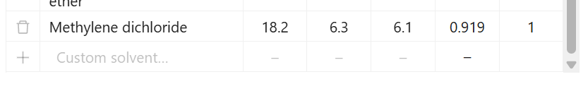
The bottom of the solvent table always shows an empty row for entering a solvent that is not in the built-in database — for example, a proprietary solvent blend or a material for which you have measured HSP values yourself.
Fill in the four editable fields in that row:
| Field | Description |
|---|---|
| Solvent | Free-text name (any label you choose) |
| δD | Dispersion Hansen parameter (MPa½) |
| δP | Polar Hansen parameter (MPa½) |
| δH | Hydrogen bonding Hansen parameter (MPa½) |
Once all four fields contain valid values, the + button in the leftmost column becomes active. Click it — or press Enter in any of the four input fields — to commit the row. The custom solvent is added to the grid with a blank Score, and the empty row resets for the next entry.
5. HSP Fitting
5.1 Running a Fit
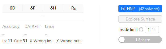
Once at least one solvent has a Score assigned, the Fit HSP button in the Fitting Panel becomes active and shows the number of scored solvents in brackets, e.g. Fit HSP (42 solvents).
Click Fit HSP to run the optimisation. The button shows a loading spinner while the calculation runs.
5.2 Fitting Parameters
Inside Limit
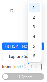
The Inside Limit selector (values 1–6) sets the minimum Score a solvent must have to be considered inside the sphere during fitting.
- Inside Limit = 1 — use with binary scoring (0/1). Any solvent scored 1 is treated as good (inside); solvents scored 0 are bad (outside).
- Inside Limit = 1–5 — solvents scoring at or above the limit are treated as inside the sphere; lower scores are outside.
This mirrors the inside_limit parameter in HSPiPy.
1 Sphere / 2 Spheres toggle
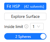
The 1 Sphere / 2 Spheres toggle controls whether the algorithm fits one or two independent HSP spheres simultaneously. Two-sphere fitting is useful for materials with bimodal solubility behaviour (e.g. some polymers or surfactants).
When two spheres are fit, the result table shows two rows (one per sphere) and both spheres are drawn on the plot.
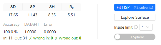
5.3 Reading the Results
Result table
| Column | Description |
|---|---|
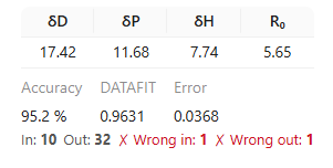
| δD | Dispersion Hansen parameter of the sphere centre (MPa½) |
| δP | Polar Hansen parameter of the sphere centre (MPa½) |
| δH | Hydrogen bonding Hansen parameter of the sphere centre (MPa½) |
| R₀ | Radius of the fitted sphere (MPa½) |
Statistics
| Metric | Description |
|---|---|
| Accuracy | Percentage of solvents correctly classified by the sphere (higher is better) |
| DATAFIT | HSPiPy's DATAFIT metric — a score from 0 to 1 reflecting fit quality (closer to 1 is better) |
| Error | Optimisation residual error (lower is better) |
Solvent counts
| Counter | Description |
|---|---|
| In | Number of scored solvents that fall inside the sphere (RED ≤ 1) |
| Out | Number of scored solvents that fall outside the sphere (RED > 1) |
| ✗ Wrong in | Solvents scored as bad (below Inside Limit) but inside the sphere — shown red if > 0 |
| ✗ Wrong out | Solvents scored as good (≥ Inside Limit) but outside the sphere — shown red if > 0 |
The RED value (Relative Energy Difference) for each solvent is shown in the RED column of the grid table after a fit. RED < 1 means the solvent is inside the sphere; RED > 1 means it is outside.
5.4 Surface Explorer
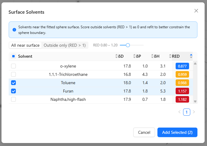
The Explore Surface button (available after a successful fit) opens the Surface Solvents modal. It queries the built-in solvent database for solvents that lie near the boundary of the fitted sphere — these are candidates that may help constrain the sphere more precisely when scored and added to the grid.
How it works
The explorer fetches all database solvents whose RED value falls within a configurable tolerance band around 1.0 (i.e., 1 − tolerance ≤ RED ≤ 1 + tolerance).
Controls
| Control | Description |
|---|---|
| Sphere selector | Shown only when two spheres are fitted; switches which sphere's surface is explored |
| All near surface / Outside only | Toggle between showing all solvents within the tolerance band, or only those with RED > 1 |
| RED range slider | Adjusts the tolerance (±0.05 to ±0.50). Wider tolerance returns more solvents |
Table columns
| Column | Description |
|---|---|
| Solvent | Solvent name (sortable) |
| δD / δP / δH | Hansen parameters (sortable) |
| RED | Relative Energy Difference, colour-coded: blue = inside (RED < 0.95), amber = on surface (0.95–1.05), red = outside (RED > 1.05) |
Workflow tip
- Run an initial fit.
- Open Surface Explorer and filter to Outside only.
- Select solvents you can test experimentally and add them to the grid.
- Score the newly added solvents (0 if they do not dissolve the material).
- Refit — the additional bad solvents outside the sphere help push the boundary inward to a more accurate result.
Select rows using the checkboxes and click Add Selected (n) to insert them into the current grid with a blank Score.
6. Visualisation
6.1 3D View
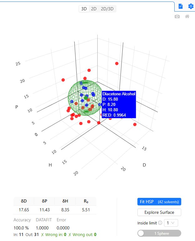
The 3D view shows all solvents as points in the Hansen solubility space (axes: D, H, P). After a fit, the HSP sphere is drawn as a green wireframe.
| Colour | Meaning |
|---|---|
| Grey (semi-transparent) | Unscored solvent |
| Blue | Good solvent (Score ≥ Inside Limit) |
| Red | Bad solvent (Score < Inside Limit, Score > 0) |
| Green wireframe + dot | Fitted HSP sphere centre |
Hovering over a point shows a tooltip with the solvent name and its δD, δP, δH coordinates. If a fit has been run, the RED value is also shown for scored solvents.
6.2 2D View
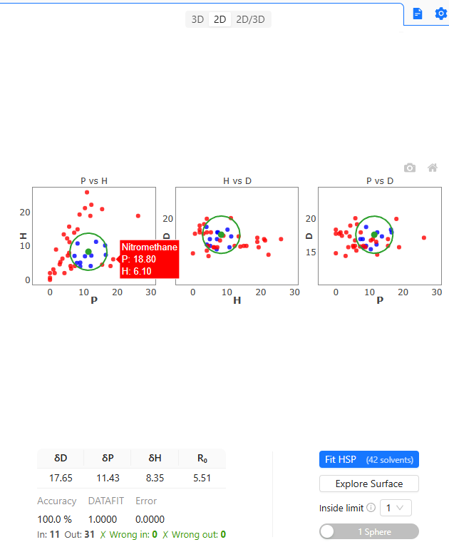
The 2D view shows three 2D projections of the solvent space side by side. This is useful for identifying which plane shows the clearest separation between good and bad solvents.
| Subplot | Axes |
|---|---|
| Left — P vs H | x = P, y = H |
| Centre — H vs D | x = H, y = D |
| Right — P vs D | x = P, y = D |
After a fit, the sphere projection appears as a green circle in each subplot. The same colour coding as the 3D view applies.
6.3 Combined 2D/3D View
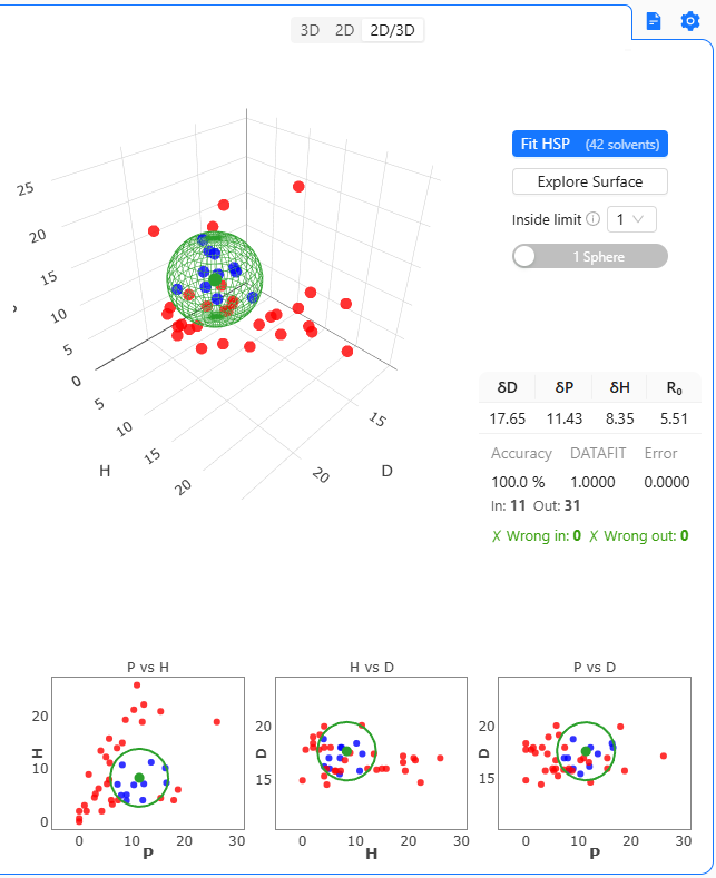
The 2D/3D mode shows both the 3D scatter plot and the three 2D subplots at the same time. The fitting panel is repositioned to the right of the 3D plot to save vertical space.
This mode is best used on wide screens or when you want to inspect both the spatial distribution and the individual plane projections simultaneously.
6.4 Interacting with the Plots
All plots are powered by Plotly and support the following interactions:
| Action | Effect |
|---|---|
| Click + drag | Rotate (3D) or pan (2D) |
| Scroll wheel | Zoom in/out |
| Double-click | Reset view to default zoom |
| Hover over point | Show solvent name and coordinates |
| Toolbar (top-right of plot) | Camera (PNG download) and Home (reset view) |
7. Settings
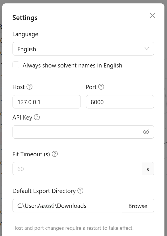
Click the settings icon in the top-right corner of the window to open the Settings modal.
Language
| Option | Language |
|---|---|
| English | English |
| Español | Spanish |
| 中文 | Simplified Chinese |
The change takes effect immediately. The selected language is persisted and restored on the next launch.
Always show solvent names in English
A checkbox directly below the language selector. When enabled, all solvent names from the built-in database are displayed in English regardless of the selected interface language. Useful when working in Spanish or Chinese but needing solvent names to match published literature or lab documentation. The setting is persisted across sessions.
Host and Port
| Field | Default | Description |
|---|---|---|
| Host | 127.0.0.1 | The network address the backend server listens on. Use 127.0.0.1 to keep it local-only (recommended). Set to 0.0.0.0 to allow connections from other devices on your network. |
| Port | 8000 | The TCP port the backend API runs on. Change this if port 8000 is already in use. |
API Key
An optional secret key that must be included in all requests to the backend API. Useful when the server is exposed beyond localhost.
Fit Timeout
Maximum number of seconds a fitting operation may run before it is abandoned and a timeout error is returned. Set to 0 to disable the limit entirely. The default is 60 seconds, which is sufficient for most datasets; very large grids or slow machines may require a higher value.
Default Export Directory
The folder that the native save dialog opens to when exporting a grid (CSV or Excel). If left empty, the system default (usually Downloads) is used. Click Browse to select a folder.
About
The Settings modal also displays the application version and links to: EULA, Privacy Policy, and Third-party Licenses.
Documentation
Click the docs icon (to the left of the settings icon) to open this user manual in your browser.
8. Troubleshooting
The application shows the splash screen for a long time
On first launch the setup dialog (language, EULA, license) appears before the backend starts — this is expected. The app polls the backend continuously with no fixed timeout. On macOS the very first launch may take longer while the system verifies the backend component. If startup takes unusually long, click Cancel to quit, then run xattr -cr /Applications/hsp-desktop.app in Terminal before relaunching. On all platforms, check that port 8000 is not in use by another application.
The EULA or language dialog keeps appearing
The language preference, EULA acceptance, and license data are each stored locally. If any of this data is cleared, the corresponding step reappears on next launch. Complete the step again to proceed normally.
My license key is not accepted
- Ensure you have copied the complete key (format:
XXXXXXXX-XXXX-XXXX-XXXX-XXXXXXXXXXXX) without leading or trailing spaces. - Check that the key has not already been used on the maximum number of allowed seats.
- Verify your internet connection — activation requires a call to the license server.
- Contact support if the issue persists.
Scores are not being saved
The Score column only stores integer values. For binary scoring use 0 or 1; for graduated scoring use 1–6. Values outside the valid range or non-numeric input are silently discarded.
The grid is considered dirty (unsaved) as soon as any score is changed — the save icon turns amber. Remember to save to the database if you want to reload the grid in a future session.
The fit produces low accuracy
- Check that the Inside Limit matches your scoring convention. For binary scoring (0/1) set Inside Limit to 1. For graduated scoring, set it to the threshold that separates good from bad solvents (commonly 3 or 4).
- A small dataset (fewer than ~6 scored solvents) gives unreliable results.
- Try the 2 Spheres mode if the good solvents appear to cluster in two distinct regions of the plot.
- Use the Surface Explorer to find additional solvents near the sphere boundary and score them to better constrain the fit.
I cannot rename or duplicate a grid
These operations require that a grid is saved in the database. A grid imported from a file or freshly created but not yet saved does not have a database ID. Save it first using the Save to DB button, then rename or duplicate.
Exported file does not open in Excel
Make sure the export format is Export as Excel (.xlsx) rather than CSV. Some regional Excel settings may require you to change the decimal separator in the CSV; the Excel export avoids this issue entirely.
The Surface Explorer returns no results
- A fit must be run before the explorer can be used. The Explore Surface button is disabled until a fit result is available.
- If the tolerance is very narrow (e.g. ±0.05), few or no solvents may fall within the band. Increase the tolerance slider.